Note

Click here to download the full example code

K-Sample Testing¶

A common problem experienced in research is the k-sample testing problem. Conceptually, it can be described as follows: consider k groups of data where each group had a different treatment. We can ask, are these groups the similar to one another or statistically different? More specifically, supposing that each group has a distribution, are these distributions equivalent to one another, or is one of them different?

If you are interested in questions of this mold, this module of the package is for you! All our tests can be found in hyppo.ksample, and will be elaborated in detail below. But before that, let's look at the mathematical formulations:

Consider random variables \(U_1, U_2, \ldots, U_k\) with distributions \(F_{U_1}, F_{U_2}, \ldots F_{U_k}\). When performing k-sample testing, we are seeing whether or not these distributions are equivalent. That is, we are testing

\[\begin{split}H_0 &: F_{U_1} = F_{U_2} = \cdots = F_{U_k} \\ H_A &: \exists \, i \neq j \text{ s.t. } F_{U_i} \neq F_{U_j}\end{split}\]

Like all the other tests within hyppo, each method has a statistic and test method. The test method is the one that returns the test statistic and p-values, among other outputs, and is the one that is used most often in the examples, tutorials, etc. The p-value returned is calculated using a permutation test using hyppo.tools.perm_test unless otherwise specified.

Specifics about how the test statistics are calculated for each in hyppo.ksample can be found the docstring of the respective test. let's look at unique properties of some of these tests:

Multivariate Analysis of Variance (MANOVA) and Hotelling¶

MANOVA is the current standard for k-sample testing in the literature. More details can be found in hyppo.ksample.MANOVA. Hotelling is 2-sample MANOVA. More details can be found in hyppo.ksample.Hotelling.

Note

Pros

Very fast
Similar to tests found in scientific literature

Cons

Not accurate when compared to other tests in most situations
Assumes data is derived from a multivariate Gaussian
Assumes data is has same covariance matrix

Neither of these test are distance based, and so do not have a compute_distance parameter and are not nonparametric, so they don't have reps nor workers. Otherwise, these test runs like any other test.

K-Sample Testing via Independence Testing¶

Nonparametric MANOVA via Independence Testing is a k-sample test that addresses the aforementioned k-sample testing problem as follow: reduce the k-sample testing problem to the independence testing problem (see Independence Testing). To solve this, we create a new matrix of concatenated inputs and a matrix that labels which of the concatenated data comes from which input [2]. Because independence tests have high finite sample testing power in some cases, this method has a number of advantages. More details can be found in hyppo.ksample.KSample. The following applies to both:

Note

If you want use 2-sample MGC, we have added that functionality to SciPy! Please see scipy.stats.multiscale_graphcorr.

Note

Pros

Highly accurate
No additional computation complexity added
Not many assumptions of the data (only must be i.i.d.)
Has fast implementations (for indep_test="Dcorr" and indep_test="Hsic")

Cons

Can be a little slower than some of the other tests in the package

The indep_test parameter accepts a string corresponding to the name of the class in the hyppo.independence. Other parameters are those in the corresponding independence test. Since this this process is nearly the same for all independence tests, we are going to use hyppo.independence.MGC as the example independence test.

from hyppo.ksample import KSample
from hyppo.tools import rot_ksamp

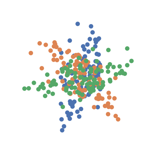
# 100 samples, 1D cubic independence simulation, 3 groups sim, 60 degree rotation, no
# noise
sims = rot_ksamp("linear", n=100, p=1, k=3, degree=[60, -60], noise=True)

The data are points simulating a 1D linear relationship between random variables \(X\) and \(Y\). It the concatenates these two matrices, and then rotates the simulation by 60 degrees, generating the second and, in this case, the third sample. It returns realizations as numpy.ndarray.

import matplotlib.pyplot as plt
import seaborn as sns

# make plots look pretty
sns.set(color_codes=True, style="white", context="talk", font_scale=1)

# look at the simulation
plt.figure(figsize=(5, 5))
for sim in sims:
    plt.scatter(sim[:, 0], sim[:, 1])
plt.xticks([])
plt.yticks([])
sns.despine(left=True, bottom=True, right=True)
plt.show()

# run k-sample test on the provided simulations. Note that *sims just unpacks the list
# we got containing our simulated data
stat, pvalue = KSample(indep_test="Dcorr").test(*sims)
print(stat, pvalue)

Out:

0.020257572395244467 0.007806778339791604

This was a general use case for the test, but there are a number of intricacies that depend on the type of independence test chosen. Those same parameters can be modified in this class. For a full list of the parameters, see the desired test in hyppo.independence and for examples on how to use it, see Independence Testing.

Distance (and Kernel) Equivalencies¶

It turns out that a number of test statistics are multiples of one another and so, their p-values are equivalent to the above K-Sample Testing via Independence Testing. [1] goes through the distance and kernel equivalencies and [2] goes through the independence and two-sample (and by extension k-sample) equivalences in far more detail.

Energy is a powerful distance-based two sample test, Distance components (DISCO) is the k-sample analogue to Energy, and Maximal mean discrepency (MMD) is a powerful kernel-based two sample test, These are equivalent to hyppo.ksample.KSample using indep_test="Dcorr" for Energy and DISCO and indep_test="Hsic" for MMD. More information can be found at hyppo.ksample.Energy, hyppo.ksample.DISCO, and hyppo.ksample.MMD. However, the test statistics have been modified to make it more in tune with other implementations.

Note

Pros

Highly accurate
Has similar test statistics to the literature
Has fast implementations

Cons

Lower power than more computationally complex algorithms

For MMD, kernels are used instead of distances with the compute_kernel parameter. Any addition, if the bias variant of the test statistic is required, then the bias parameter can be set to True. In general, we do not recommend doing this. Otherwise, these tests runs like any other test.

Smooth Characteristic Function Test¶

The Smooth Characteristic Function Test (Smooth CF), is a form of non-parametric two-sample tests. The Smooth CF test utilizes smoothed empirical characteristic functions to represent two data distributions. Characteristic functions completely define the probability distribution of a random variable. In hypothesis testing, it is useful to estimate characteristic functions for given data. However, empirical characteristic functions can be very complex and therefore expensive to compute. The smooth characteristic function can serve as a heuristic in place of the empirical function which is much faster w.r.t. computation times. More information can be found at hyppo.ksample.SmoothCFTest.

Note

Pros

Very fast computation time
Faster than current, state-of-the-art quadratic-time kernel-based tests

Cons

Heuristic method, checking more frequencies will give more power.

This test is also initialized with the num_randfreq parameter. This parameter can be thought of as the degrees of freedom associated with the test and also dictates the number of test points used in the test (see hyppo.ksample.SmoothCFTest). If data is kept constant, increasing the magnitude of this parameter will generally result in larger magnitude test statistics while magnitude of the p-value will fluctuate:

import numpy as np
from hyppo.ksample import SmoothCFTest

np.random.seed(1234)
x = np.random.randn(500, 10)
y = np.random.randn(500, 10)

stat1, pvalue1 = SmoothCFTest(num_randfreq=5).test(x, y, random_state=1234)
stat2, pvalue2 = SmoothCFTest(num_randfreq=10).test(x, y, random_state=1234)

print("5 degrees of freedom (stat, pval):\n", stat1, pvalue1)
print("10 degrees of freedom (stat, pval):\n", stat2, pvalue2)

Out:

degrees of freedom (stat, pval):
698068715588362 0.9104136782024711
degrees of freedom (stat, pval):
494540898474115 0.8045631415568775

Mean Embedding Test¶

The Mean Embedding Test is another non-parametric two-sample statistical test. This test is based on analytic mean embeddings of data distributions in a reproducing kernel hilbert space (RKHS). Hilbert spaces allow the representation of functions as points; thus, if mean embeddings can be determined for two data distributions then the distance between these two distributions in the hilbert space can be determined. In other words, the RKHS allows the mapping of probability measures into a finite dimensional Euclidean space. More details can be found at hyppo.ksample.MeanEmbeddingTest.

Note

Pros

Very fast computation time
Faster than current, state-of-the-art quadratic-time kernel-based tests

Cons

Heuristic method, checking more frequencies will give more power.

This test is also initialized with the num_randfreq parameter. This parameter can be thought ofas the degrees of freedom associated with the test and also dictates the number of test points used in the test (see hyppo.ksample.MeanEmbeddingTest). If data is kept constant, increasing the magnitude of this parameter will generally result in larger magnitude test statistics while magnitude of the p-value will fluctuate:

from hyppo.ksample import MeanEmbeddingTest

np.random.seed(1234)
x = np.random.randn(500, 10)
y = np.random.randn(500, 10)

stat1, pval1 = MeanEmbeddingTest(num_randfreq=5).test(x, y, random_state=1234)
stat2, pval2 = MeanEmbeddingTest(num_randfreq=10).test(x, y, random_state=1234)

print("5 degrees of freedom (stat, pval):\n", stat1, pval1)
print("10 degrees of freedom (stat, pval):\n", stat2, pval2)

Out:

degrees of freedom (stat, pval):
32713968958162 0.377273001086016
degrees of freedom (stat, pval):
150092396142151 0.42742539627581594

Univariate-Based Test¶

The Heller Heller Gorfine (HHG) 2-Sample Test is a non-parametric two-sample statistical test. This test is based on testing the independence of the distances of sample vectors from a center point by a univariate K-sample test. If the distribution of samples differs across categories, then so does the distribution of distances of the vectors from almost every point z. The univariate test used is the Kolmogorov-Smirnov 2-sample Test, which looks at the largest absolute deviation between the cumulative distribution functions of the samples. More info can found at hyppo.ksample.KSampleHHG.

Note

Pros

Very fast computation time

Cons

Lower power than more computationally complex algorithms
Inherits the assumptions of the KS univariate test

from hyppo.ksample import KSampleHHG

np.random.seed(1234)

x, y = rot_ksamp("linear", n=100, p=1, k=2, noise=False)

stat, pvalue = KSampleHHG().test(x, y)
print(stat, pvalue)

Out:

0.5757575757575758 3.3189957106557175e-13

Total running time of the script: ( 0 minutes 0.810 seconds)

Gallery generated by Sphinx-Gallery

D-Variate Independence Testing

Time Series Testing