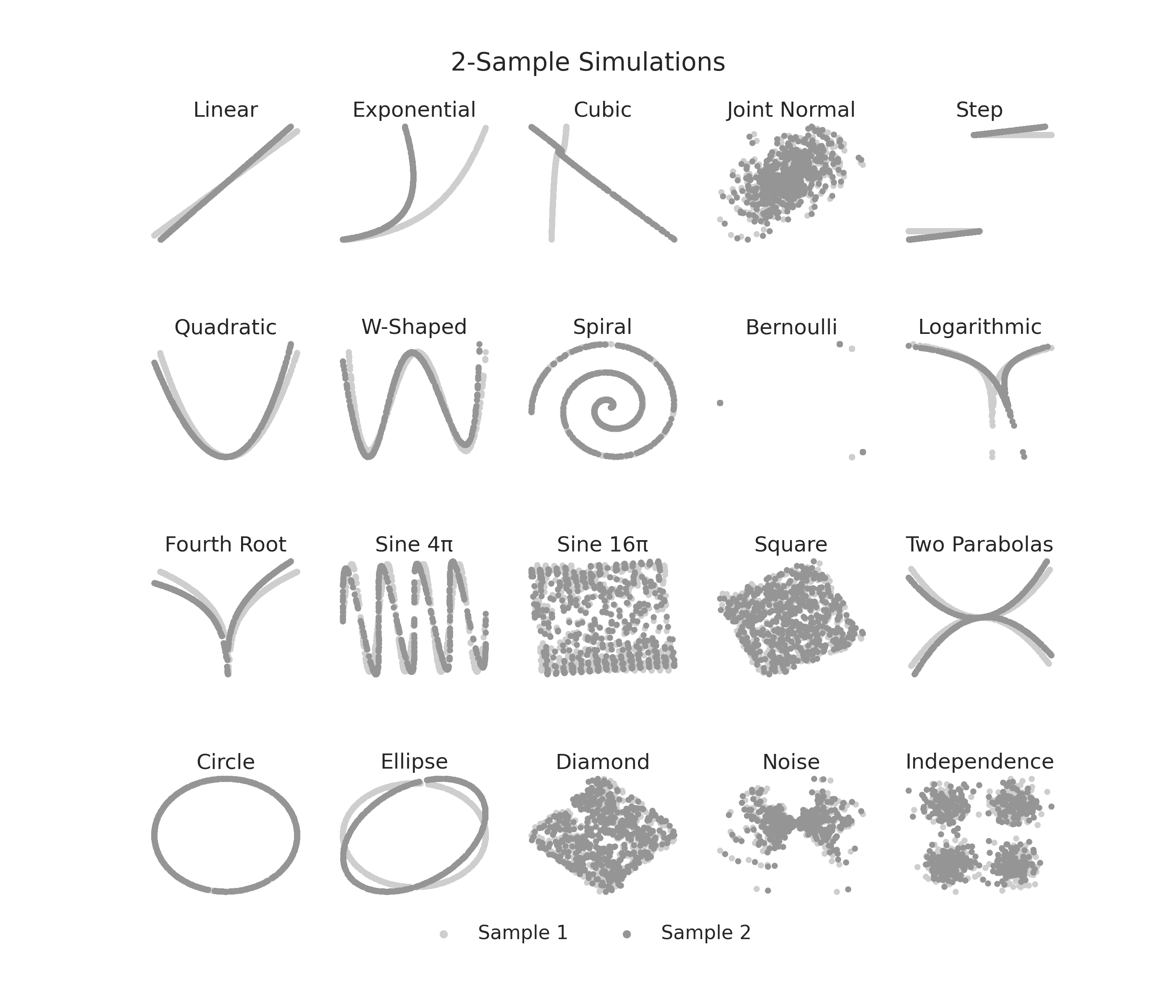
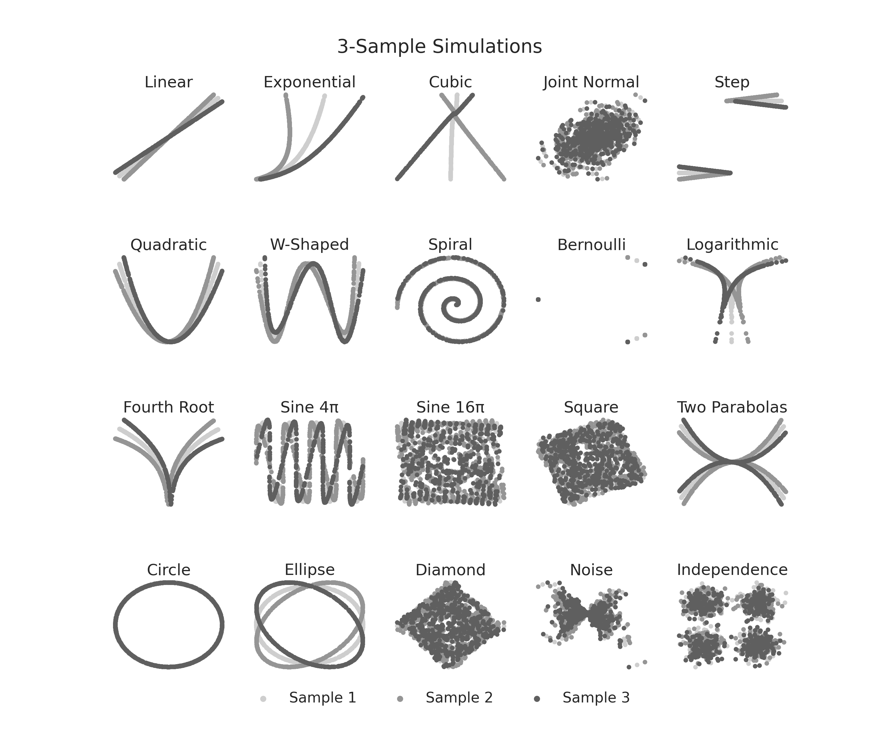
K-Sample Sims

K-sample simulations are found in hyppo.tools. Here, we visualize what these simulations look like. The original simulation and rotated simulation are shown. Note that since these are noise-free, we do not see any rotation due to the rotational symmetry of the simulation.

• 
• 

import matplotlib.pyplot as plt
import seaborn as sns
from hyppo.tools import SIMULATIONS, rot_ksamp

# make plots look pretty
sns.set(color_codes=True, style="white", context="talk", font_scale=2)
PALETTE = sns.color_palette("Greys", n_colors=9)
sns.set_palette(PALETTE[2::2])

# constants
N = 500  # sample size
P = 1  # dimensionality
DEGREE = [5, -5]  # angle

# simulation titles
SIM_TITLES = [
    "Linear",
    "Exponential",
    "Cubic",
    "Joint Normal",
    "Step",
    "Quadratic",
    "W-Shaped",
    "Spiral",
    "Bernoulli",
    "Logarithmic",
    "Fourth Root",
    "Sine 4\u03C0",
    "Sine 16\u03C0",
    "Square",
    "Two Parabolas",
    "Circle",
    "Ellipse",
    "Diamond",
    "Noise",
    "Independence",
]


# make a function that runs the code depending on the simulation
def plot_sims(k=2, degree=DEGREE):
    """Plot simulations"""
    fig, ax = plt.subplots(nrows=4, ncols=5, figsize=(28, 24))

    plt.suptitle("{}-Sample Simulations".format(k), y=0.93, va="baseline")

    count = 0
    for i, row in enumerate(ax):
        for j, col in enumerate(row):
            count = 5 * i + j
            sim_title = SIM_TITLES[count]
            sim = list(SIMULATIONS.keys())[count]

            # rotated k-sample simulation
            sims = rot_ksamp(sim, N, P, k=k, degree=degree, noise=False)

            # plot the nose and noise-free sims
            for index in range(len(sims)):
                col.scatter(
                    sims[index][:, 0],
                    sims[index][:, 1],
                    label="Sample {}".format(index + 1),
                )

            # make the plot look pretty
            col.set_title("{}".format(sim_title))
            col.set_xticks([])
            col.set_yticks([])
            sns.despine(left=True, bottom=True, right=True)

    leg = plt.legend(
        bbox_to_anchor=(0.5, 0.1),
        bbox_transform=plt.gcf().transFigure,
        ncol=5,
        loc="upper center",
    )
    leg.get_frame().set_linewidth(0.0)
    for legobj in leg.legendHandles:
        legobj.set_linewidth(5.0)
    plt.subplots_adjust(hspace=0.75)


# run the created function for the simultions for 2 sample and 3 sample
# and run for the guassian simulations
plot_sims(k=2, degree=DEGREE[0])
plot_sims(k=3, degree=DEGREE)

previous

Guassian Sims

next

Time-Series Sims