Time Series Testing

A common problem, especially in the realm of data such as fMRI images, is identifying causality within time series data. This is difficult and sometimes impossible to do among multivarate and nonlinear data.

If you are interested in questions of this mold, this module of the package is for you! All our tests can be found in hyppo.time_series, and will be elaborated in detail below. But before that, let's look at the mathematical formulations:

Let \(\mathbb{N}\) be the non-negative integers \({0, 1, 2, \ldots}\), and \(\mathbb{R}\) be the real line \((−\infty, \infty)\). Let \(F_X\), \(F_Y\), and \(F_{XY}\) represent the marginal and joint distributions of random variables \(X\) and \(Y\), whose realizations exist in \(\mathcal{X}\) and \(\mathcal{Y}\), respectively. Similarly, Let \(F_X\), \(F_Y\), and \(F_{(X_t, Y_s)}\) represent the marginal and joint distributions of the time-indexed random variables \(X_t\) and \(Y_s\) at timesteps \(t\) and \(s\). For this work, assume \(\mathcal{X} = \mathbb{R}^p\) and \(\mathcal{Y} = \mathbb{R}^q\) for \(p, q > 0\). Finally, let \(\{(X_t, Y_t)\}_{t = -\infty}^\infty\) represent the full, jointly-sampled time series, structured as a countably long list of observations \((X_t, Y_t)\). Consider a strictly stationary time series \(\{(X_t, Y_t)\}_{t = -\infty}^\infty\), with the observed sample \(\{(X_1, Y_1), \ldots, (X_n, Y_n)\}\). Choose some \(M \in \mathbb{N}\), the maximum_lag hyperparameter. We test the independence of two series via the following hypothesis.

\[\begin{split}H_0: F_{(X_t,Y_{t-j})} &= F_{X_t} F_{Y_{t-j}} \text{ for each } j \in {0, 1, \ldots, M} \\ H_A: F_{(X_t,Y_{t-j})} &\neq F_{X_t} F_{Y_{t-j}} \text{ for some } j \in {0, 1, \ldots, M}\end{split}\]

The null hypothesis implies that for any \((M + 1)\)-length stretch in the time series, \(X_t\) is pairwise independent of present and past values \(Y_{t - j}\) spaced \(j\) timesteps away (including \(j = 0\)). A corresponding test for whether \(Y_t\) is dependent on past values of \(X_t\) is available by swapping the labels of each time series. Finally, the hyperparameter \(M\) governs the maximum number of timesteps in the past for which we check the influence of \(Y_{t - j}\) on \(X_t\). This \(M\) can be chosen for computation considerations, as well as for specific subject matter purposes, e.g. a signal from one region of the brain might only influence be able to influence another within 20 time steps implies \(M = 20\).

Like all the other tests within hyppo, each method has a statistic and test method. The test method is the one that returns the test statistic and p-values, among other outputs, and is the one that is used most often in the examples, tutorials, etc. The p-value returned is calculated using a permutation test.

Cross multiscale graph correlation (MGCX) and cross distance correlation (DcorrX) are time series tests of independence. They are a more powerful alternative to pairwise Pearson's correlation comparisons that are the standard in the literature, and is multivariate and distance based. More details can be found in hyppo.time_series.MGCX and hyppo.time_series.DcorrX.

Note

Pros

• Very accurate

• Operates of multivariate data

Cons

• Slower than pairwise Pearson's correlation

Each class has a max_lag parameter that indicates the maximum number of lags to check between an inputs x and the shifted y. Both statistic functions return opt_lag, while MGCX returns the optimal scale (see hyppo.independence.MGC for more info).

As an example, let's generate some simulated data using hyppo.tools.indep_ar:

from hyppo.tools import indep_ar

# 40 samples, Independence AR, lag = 1
x, y = indep_ar(40)

The data are points simulating an independent AR(1) process and returns realizations as numpy.ndarray:

import matplotlib.pyplot as plt
import seaborn as sns

# make plots look pretty
sns.set(color_codes=True, style="white", context="talk", font_scale=1)

# look at the simulation
n = x.shape[0]
t = range(1, n + 1)
fig, (ax1, ax2) = plt.subplots(1, 2, figsize=(15, 7.5))
ax1.plot(t, x)
ax1.plot(t, y)
ax2.scatter(x, y)
ax1.legend(["X_t", "Y_t"], loc="upper left", prop={"size": 12})
ax1.set_xlabel(r"$t$")
ax2.set_xlabel(r"$X_t$")
ax2.set_ylabel(r"$Y_t$")
fig.suptitle("Independent AR (lag=1)")
plt.axis("equal")
plt.show()

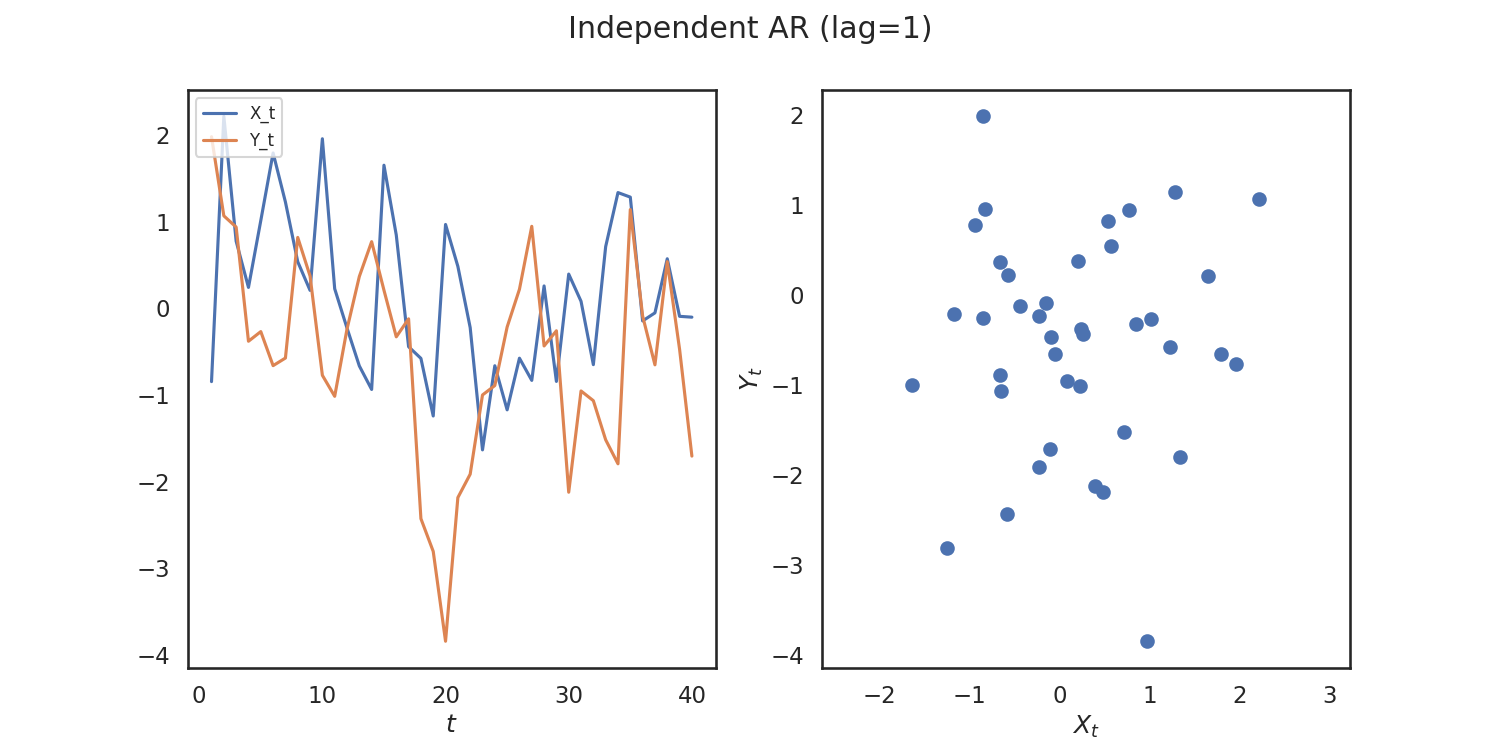
Since the simulations are independent, we would expect to see a high p-value. We can verify whether or not we can see a trend within the data by running a time-series independence test. Let's use MGCX We have to import it, and then run the test.

from hyppo.time_series import DcorrX

stat, pvalue, _ = DcorrX(max_lag=0).test(x, y)
print(stat, pvalue)

Out:

0.0 1.0

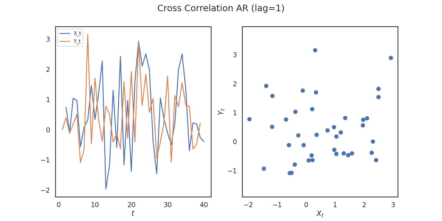
So, we verify that we get a high p-value! Let's repeat this process again for simulations that are correlated. We woulld expect a low p-value in this case.

from hyppo.tools import cross_corr_ar

# 40 samples, Cross Correlation AR, lag = 1
x, y = cross_corr_ar(40)

# stuff to make the plot and make it look nice
n = x.shape[0]
t = range(1, n + 1)
fig, (ax1, ax2) = plt.subplots(1, 2, figsize=(15, 7.5))
ax1.plot(t[1:n], x[1:n])
ax1.plot(t[0 : (n - 1)], y[0 : (n - 1)])
ax2.scatter(x, y)
ax1.legend(["X_t", "Y_t"], loc="upper left", prop={"size": 12})
ax1.set_xlabel(r"$t$")
ax2.set_xlabel(r"$X_t$")
ax2.set_ylabel(r"$Y_t$")
fig.suptitle("Cross Correlation AR (lag=1)")
plt.axis("equal")
plt.show()

stat, pvalue, _ = DcorrX(max_lag=1).test(x, y)
print(stat, pvalue)

Out:

0.09777788778538327 0.07692307692307693

previous

K-Sample Testing

next

Discriminability Testing