Note
Click here to download the full example code
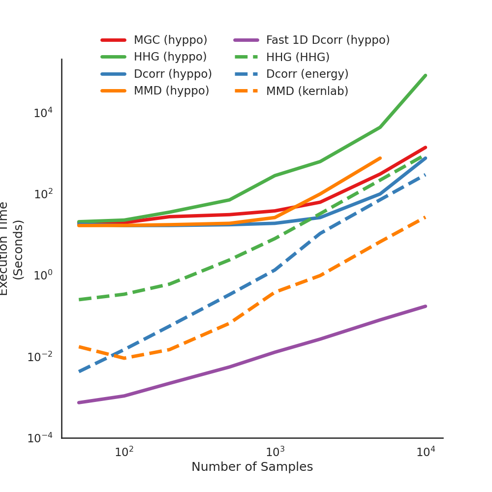
1D Performance Comparisons
There are few implementations in hyppo.independence the have implementations
in R. Here, we compare the test statistics between the R-generated values and our
package values. As you can see, there is a minimum difference between test statistics.
import os
import sys
import timeit

import matplotlib.pyplot as plt
import numpy as np
import seaborn as sns
from hyppo.independence import HHG, MGC, Dcorr
from hyppo.ksample import MMD
from hyppo.tools import linear

sys.path.append(os.path.realpath(".."))

# make plots look pretty
sns.set(color_codes=True, style="white", context="talk", font_scale=1)
PALETTE = sns.color_palette("Set1")
sns.set_palette(PALETTE[1:])

# constants
N = [50, 100, 200, 500, 1000, 2000, 5000, 10000]  # sample sizes
FONTSIZE = 20

# tests
TESTS = {"indep": [Dcorr, MGC, HHG], "ksample": [MMD], "fast": [Dcorr]}


# function runs wall time estimates using timeit (for python)
def estimate_wall_times(test_type, tests, **kwargs):
    for test in tests:
        times = []
        for n in N:
            x, y = linear(n, 1, noise=True)
            # numba is a JIT compiler, run code to cache first, then time
            _ = test().test(x, y, workers=-1, **kwargs)
            start_time = timeit.default_timer()
            _ = test().test(x, y, workers=-1, **kwargs)
            times.append(timeit.default_timer() - start_time)
        np.savetxt(
            "../benchmarks/perf/{}_{}.csv".format(test_type, test.__name__),
            times,
            delimiter=",",
        )
    return times


# compute wall times, uncomment to recompute
# kwargs = {}
# for test_type in TESTS.keys():
#     if test_type == "fast":
#         kwargs["auto"] = True
#     estimate_wall_times(test_type, TESTS[test_type], **kwargs)

# Dictionary of test colors and labels
TEST_METADATA = {
    "MGC": {"test_name": "MGC (hyppo)", "color": "#e41a1c"},
    "HHG": {"test_name": "HHG (hyppo)", "color": "#4daf4a"},
    "Dcorr": {"test_name": "Dcorr (hyppo)", "color": "#377eb8"},
    "ksample_Hsic": {"test_name": "MMD (hyppo)", "color": "#ff7f00"},
    "fast_Dcorr": {"test_name": "Fast 1D Dcorr (hyppo)", "color": "#984ea3"},
    "HHG_hhg": {"test_name": "HHG (HHG)", "color": "#4daf4a"},
    "Dcorr_energy": {"test_name": "Dcorr (energy)", "color": "#377eb8"},
    "Dcorr_kernlab": {"test_name": "MMD (kernlab)", "color": "#ff7f00"},
}


def plot_wall_times():
    _ = plt.figure(figsize=(10, 10))
    ax = plt.subplot(111)

    i = 0
    kwargs = {}
    for file_name, metadata in TEST_METADATA.items():
        test_times = np.genfromtxt(
            "../benchmarks/perf/{}.csv".format(file_name), delimiter=","
        )

        if file_name in ["HHG_hhg", "Dcorr_energy", "Dcorr_kernlab"]:
            kwargs = {"linestyle": "dashed"}
        ax.plot(
            N,
            test_times,
            color=metadata["color"],
            label=metadata["test_name"],
            lw=5,
            **kwargs
        )
        i += 1

    ax.spines["top"].set_visible(False)
    ax.spines["right"].set_visible(False)
    ax.set_xlabel("Number of Samples")
    ax.set_ylabel("Execution Time\n(Seconds)")
    ax.set_xscale("log")
    ax.set_yscale("log")
    ax.set_xticks([1e2, 1e3, 1e4])
    ax.set_yticks([1e-4, 1e-2, 1e0, 1e2, 1e4])

    leg = plt.legend(
        bbox_to_anchor=(0.5, 0.95),
        bbox_transform=plt.gcf().transFigure,
        ncol=2,
        loc="upper center",
    )
    leg.get_frame().set_linewidth(0.0)
    for legobj in leg.legend_handles:
        legobj.set_linewidth(5.0)


# plot the wall times
plot_wall_times()
The following shows the code that was used to compute the R test statistics. Certain lines were commented out depending on whether or not they were useful.
rm(list=ls())

require("energy")
require("kernlab")
require("mgc")
require("HHG")
require("microbenchmark")

num_samples_range = c(50, 100, 200, 500, 1000, 2000, 5000, 10000)
linear_data <- list()
i <- 1
for (num_samples in num_samples_range){
  data <- mgc.sims.linear(num_samples, 1)
  x <- data$X
  y <- data$Y
  times = seq(1, 3, by=1)
  executions <- list()
  for (t in times){
    # x <- as.matrix(dist((x), diag = TRUE, upper = TRUE))
    # y <- as.matrix(dist((y), diag = TRUE, upper = TRUE))

    # best of 5 executions
    # time <- microbenchmark(kmmd(x, y, ntimes=1000), times=1, unit="secs")
    # time <- microbenchmark(dcor.test(x, y, R=1000), times=1, unit="secs")
    # time <- microbenchmark(dcor.test(x, y, R=1000), times=1, unit="secs")
    time <- microbenchmark(dcor2d(x, y), times=1, unit="secs")
    # time <- microbenchmark(hhg.test(x, y, nr.perm=1000), times=1, unit="secs")
    executions <- c(executions, list(time[1, 2]/(10^9)))
  }
  linear_data <- c(linear_data, list(sapply(executions, mean)))

  print("Finished")
  i <- i + 1
}

df <- data.frame(
   matrix(unlist(linear_data), nrow=length(linear_data), byrow=T),
   stringsAsFactors=FALSE
 )
write.csv(df, row.names=FALSE)
Total running time of the script: ( 0 minutes 0.197 seconds)